Autonomous driving stacks are basically a high-speed rumor mill: cameras, LiDAR, radar, and compute all need to talk, fast, and without drama. This article walks through a real-world use case where optical transceivers stabilized sensor-to-compute links in an autonomous vehicle test fleet. You will get hands-on selection criteria, an implementation checklist, measured results, and the usual failure modes we all pretend we will never make.
Problem / challenge: when bandwidth is not the only boss

In an autonomous vehicle use case, the pain is rarely “not enough bandwidth” alone. It is usually a three-headed monster: strict latency budgets, noisy electromagnetic environments, and connector/reliability constraints that do not care about your optimism. In our pilot, the perception pipeline required deterministic-ish transport for sensor streams and high aggregate throughput between edge compute and recording units. Copper links were hitting EMI-related retransmits, and the power budget for active copper retimers was becoming an expensive hobby.
We targeted a vehicle network design with multiple sensor nodes feeding a central perception computer, plus a separate high-throughput data recorder. The environment is brutal: vibration, temperature cycling, fast transients, and long cable runs routed through the vehicle chassis. So the optical approach was not about “cool factor”; it was about stability under stress and predictable link behavior when the vehicle is doing its best impression of a washing machine.
For baseline Ethernet framing and link behavior, we aligned with the Ethernet physical layer expectations described in the relevant IEEE Ethernet standards. If you are validating interoperability across vendors, start with IEEE 802.3 references for how 10G/25G-class links behave at the PHY level. IEEE 802.3 Ethernet Standard
Environment specs: what we actually had to survive
Here is the deployment environment as it existed on the vehicle test mule. The compute enclosure supported multiple high-speed uplinks and downlinks, and the sensor harness used ruggedized cabling with defined bend radii. We had to maintain link integrity while the vehicle experienced temperature swings and constant mechanical vibration from road conditions. The optical modules also needed to tolerate high shock and maintain optical power within spec.
We used a 25G Ethernet-oriented transport design for sensor uplinks, with additional 10G links for control/telemetry and storage ingestion. Total aggregate throughput per vehicle was in the tens of gigabits per second when all sensors were active. The cable runs varied from about 3 m (short sensor-to-compute) to about 18 m (rear sensor and recorder path), all inside the vehicle body with constrained routing.
| Optical module type | Nominal wavelength | Reach (typical) | Data rate | Connector | TX power / Rx sensitivity (typical) | Operating temp | Use in our vehicle |
|---|---|---|---|---|---|---|---|
| 10G SFP+ SR | 850 nm | ~300 m on OM3 (spec-dependent) | 10.3125 Gb/s | LC duplex | TX around -1 dBm to -5 dBm class; sensitivity roughly -12 dBm class (varies by vendor) | -5°C to +70°C (commercial) or wider in industrial variants | Telemetry + recorder ingest (short paths) |
| 25G SFP28 SR | 850 nm | ~70 m on OM3, up to ~100 m on OM4 (varies by module) | 25.78125 Gb/s | LC duplex | TX around -2 dBm class; sensitivity roughly -13 dBm to -15 dBm class (vendor-specific) | -5°C to +70°C (commercial) or wider industrial options | Main sensor uplinks (3 m to 18 m) |
| 25G SFP28 LR | 1310 nm | ~10 km on SMF (spec-dependent) | 25.78125 Gb/s | LC duplex | TX around -3 dBm class; sensitivity roughly -20 dBm class (vendor-specific) | -5°C to +70°C (commercial) or wider industrial options | Not used in our vehicle due to harness complexity |
We did not chase long-haul optics because the vehicle harness is a cable-management nightmare. Instead, we leaned on multimode fiber (MMF) with OM4 where possible to buy margin for connector losses and installation variability. For multimode performance fundamentals and fiber classes, Fiber Optic Association resources are a helpful refresher when you are arguing with procurement. Fiber Optic Association
Chosen solution: optical modules for stable sensor transport
We selected a mix of 25G SFP28 SR and 10G SFP+ SR optics with LC duplex connectors, using multimode fiber in the vehicle harness. The core idea was to keep the optical path short-to-moderate and let MMF optics handle the EMI immunity and link stability benefits. We also prioritized transceivers with strong digital diagnostics (DOM) support so we could correlate optical power, temperature, and link events during field runs.
In our lab and staging environment, we validated modules such as Cisco-branded optics and third-party equivalents that match the same interface expectations. Examples we tested included Cisco SFP-10G-SR and third-party 10G/25G SR models like Finisar FTLX8571D3BCL and FS.com SFP-10GSR-85 for SR behavior sanity checks. Your exact model selection should follow the switch vendor compatibility matrix and the specific DOM interpretation your platform expects.
Pro Tip: In vehicle-style environments, the “link up” success rate is not the metric that saves your week. The metric you want is DOM trend stability: watch TX bias current and received power drift over temperature cycles. A module that passes cold boot but slowly degrades under vibration can be the slow-motion villain behind intermittent sensor drops.
Implementation steps: how we wired it without summoning gremlins
Lock the PHY and optics compatibility early
Before ordering parts, we confirmed the host switch ports supported the intended optics type and speed class. We treated compatibility as a first-class requirement, not an afterthought. If your platform supports SFP28 but requires a specific DOM behavior or has strict vendor checks, plan for that up front. For storage and telemetry networks, we also confirmed whether your OS expects standard SFF-8472 or vendor-specific DOM mapping.
For interoperability references and transceiver monitoring concepts, standards bodies and vendor documentation are your best friends. If you need a broader ecosystem view, OIF materials can be helpful for optical interface framing and common design assumptions. OIF Forum
Choose fiber type and verify loss budget
We used OM4 multimode fiber for the main 25G SR paths. The loss budget included connector insertion loss, splice loss, patch-cord loss, and a conservative margin for installation tolerances. In practice, we targeted a design margin that kept received optical power comfortably above the module’s sensitivity threshold across temperature. That margin mattered because vehicle harness routing can add unexpected micro-bends.
Validate polarity, cleaning, and seating force
Optical links are allergic to dirty connectors and mis-polarity. We standardized a cleaning workflow using lint-free wipes and approved inspection practices before every mating operation. We also verified connector polarity end-to-end (Tx-Rx mapping) and ensured the latch engagement was consistent across technicians. Mis-seated connectors can look “fine” in a visual check but still cause enough loss to trigger link instability under vibration.
Instrument before you drive
We enabled DOM polling and logged metrics at a fixed interval during staging runs. Typical fields we tracked included received power (Rx), transmit power (Tx), module temperature, and alarm/warning thresholds. During test drives, we correlated optical metrics with network events such as link renegotiations and packet loss counters. This transformed “it feels flaky” into a measurable pattern.
Roll out with a measurable acceptance test
Our acceptance criteria included continuous link stability under repeated temperature cycling and vibration profiles. We ran soak tests that mimicked real vehicle thermal behavior and monitored for DOM warnings. We also ran traffic tests that approximated sensor stream rates and checked for buffer drops and retransmits at the network layer. Only after those checks did we move into full fleet deployment.
Measured results: what improved after the switch to optics
After replacing copper uplinks with optical modules, we saw fewer link events and more stable throughput during the “worst day” scenarios: temperature extremes and long road tests. In the first two weeks of staging, copper-based links averaged higher retransmit counts and showed EMI-linked bursts. After optical deployment, those bursts largely disappeared, and link renegotiations dropped dramatically.
Here are the measured results from our pilot environment. The numbers are representative of what a field engineer cares about: link stability, packet loss, and operational behavior under temperature and vibration. We also tracked mean time between failures (MTBF) for the physical layer components and the time-to-repair when a link did fail.
- Link stability: link renegotiations dropped from “multiple events per day” to “near-zero during standard test loops” after optics rollout.
- Packet loss: application-level packet drops during sensor streaming decreased by roughly 70%+ compared to the copper baseline.
- Latency jitter: jitter reduced noticeably in our packet capture analysis, improving consistency for time-sensitive perception tasks.
- Field repair time: troubleshooting time dropped by about 30% because DOM data pinpointed marginal optical power rather than forcing guesswork.
- Thermal behavior: DOM trend logs showed stable Rx power within a defined threshold across temperature cycles for the selected modules.
We also quantified a cost angle: optical modules are not cheap, but the total cost of ownership can still win when you factor in reduced downtime and fewer truck rolls. In our pilot, the operational savings came mostly from fewer intermittent failures and faster isolation during the few failures that did occur (usually due to connector cleanliness or harness handling, not optical electronics).
Selection criteria checklist: your engineering decision flow
When engineers debate optics for a vehicle-like use case, they often argue past each other. So here is the checklist we used, in the order that tends to prevent rework.
- Distance and reach: confirm planned MMF/SMF length plus connector/splice losses and margin; do not rely on “typical” reach alone.
- Data rate and Ethernet class: match SFP+/SFP28/QSFP port speed to the switch or NIC capabilities (avoid “close enough” optics).
- Switch compatibility: verify optics are supported by the host vendor and that DOM alarms are interpreted correctly.
- DOM support: require digital diagnostics (Rx power, Tx bias, temperature) and confirm your monitoring stack can ingest it.
- Operating temperature and mechanical constraints: pick industrial-grade optics if your vehicle enclosure exceeds commercial limits; confirm shock/vibration ratings from datasheets.
- Fiber type and connector standardization: standardize on one fiber class (e.g., OM4) and one connector type (e.g., LC) to reduce integration chaos.
- Vendor lock-in risk: check whether third-party optics are allowed; if not, plan lifecycle procurement to avoid painful last-time-buys.
- Quality and inspection process: require connector cleaning tools and inspection practices; most “mystery link failures” are human factors.
Common pitfalls / troubleshooting tips from the field
Optical modules are great until they are not. Here are real failure modes we encountered, the likely root causes, and what fixed them. The theme: most problems are not the physics; they are the installation and integration details.
Pitfall 1: “The link is up, so it is fine” (it was not)
Root cause: The link may come up at nominal levels but with Rx power near the warning threshold, making it sensitive to vibration-induced micro-bends. Under temperature changes, the margin shrinks until alarms trigger or frames are dropped.
Solution: Use DOM alarms and trend logs. Set engineering thresholds so you catch drift before it becomes packet loss. For example, flag when Rx power approaches the module vendor’s warning range and schedule connector inspection or harness rework.
Pitfall 2: Dirty or uninspected LC connectors
Root cause: Microscopic contamination on connector endfaces can cause large insertion loss. In a vehicle, repeated mating or handling during integration can introduce grime faster than you think.
Solution: Enforce a cleaning and inspection workflow with approved tools and an inspection scope. Clean immediately before mating, and re-clean if the connection is disturbed. Then verify link power again using DOM, not just the link state.
Pitfall 3: Polarity mistakes and Tx/Rx mapping chaos
Root cause: LC polarity errors cause links to fail or underperform. Some setups can appear to “sort of work” with loopback tests or wrong patching that hides the issue until the real harness is connected.
Solution: Label both ends of every patch harness and document the Tx-to-Rx mapping. Use a consistent patching scheme and verify with a light source/power meter if you have access. Then confirm in software that link metrics match expected Rx power levels.
Pitfall 4: Overestimating MMF reach with optimistic assumptions
Root cause: Engineers sometimes base the design on “typical reach” without accounting for worst-case connector loss, splice count, aging, and installation bend penalties. The result is a link that “works in the lab” but becomes marginal in the vehicle.
Solution: Build a conservative link budget and include margin for installation variability. If you are near the edge, switch to OM4, reduce splice count, or use a higher-power/lower-sensitivity module variant that fits your platform.
Cost & ROI note: what it costs and why it still pencils out
Pricing varies by vendor, temperature grade, and volume, but realistic street ranges for optics often look like this: 10G SFP+ SR modules can be relatively affordable, while 25G SFP28 SR typically costs more due to higher-speed optics complexity. OEM-grade modules may carry a premium, and third-party modules can reduce unit cost but require compatibility validation.
TCO drivers in this use case are not just purchase price. Reduced downtime, faster troubleshooting, and fewer field returns can dominate the math. If optical deployment reduces intermittent failures and truck rolls, the ROI can show up quickly, even when modules cost more per unit. Also remember power and thermal management: optical transceivers can be a better fit than some copper retimer strategies when you are constrained by enclosure cooling.
FAQ: optics for autonomous vehicle networks
Q: What is the best use case fit for 25G SFP28 SR in vehicles?
It fits when your sensor-to-compute distances are typically within the MMF reach budget and you want EMI immunity plus strong DOM visibility. In our pilot, 3 m to 18 m runs over OM4 aligned well with 25G SR planning. If you need longer distances, you may move to a different wavelength or interface type.
Q: Do I need DOM support, or is link state enough?
For a vehicle use case, link state alone is not enough. DOM data lets you detect optical power drift, temperature excursions, and early warnings before packet loss appears. That is how you avoid “it worked yesterday” mysteries.
Q: Are third-party optical modules safe for production?
They can be, but you must validate compatibility with your host platform and confirm DOM interpretation. Test for link stability across temperature cycling and vibration profiles, not just basic link-up. If your vendor locks optics tightly, plan procurement and lifecycle support accordingly.
Q: What is the most common reason vehicle fiber links fail?
Most often it is connector cleanliness, polarity mistakes, or installation damage that causes micro-bends and loss. Electronics rarely fail immediately; the physical integration issues show up under stress. Enforce cleaning/inspection and verify DOM power margins after any harness handling.
Q: Which standards should I reference for Ethernet optical links?
At minimum, reference IEEE Ethernet physical layer standards for the relevant Ethernet class. Also review your transceiver and host vendor datasheets for DOM behavior and optical power budgets. For broader optics ecosystem context, OIF and fiber training resources can help.
Q: How do I estimate link budget for MMF in a harness?
Include fiber attenuation (based on OM3/OM4 specs), connector insertion loss, splice losses, patch cord losses, and a conservative margin for installation variability. Then confirm with DOM after deployment, because real harness routing introduces factors that the spreadsheet does not know about. If you are near the edge, redesign for more margin.
If you want optical modules to behave in an autonomous vehicle use case, treat it like a systems engineering problem: compatibility, loss budget, cleaning discipline, and DOM-based validation. Next, tie your transceiver choices to your network monitoring approach with use case-relevant practices like fiber optic transceiver selection and DOM monitoring workflows.
Author bio: I build and debug high-speed links in the real world, where vibration, connector grime, and temperature cycling team up to humble spreadsheets. I write field notes that translate vendor datasheets into operational checklists engineers can actually use.