AI infrastructure keeps pushing Ethernet and optical links into tighter power budgets and more aggressive thermal envelopes. This article helps network architects and data center engineers decide between active solutions and passive optical approaches by walking through a real deployment case, including measured results and operational lessons. You will get practical selection criteria, troubleshooting pitfalls, and a spec comparison you can use during procurement and acceptance testing.

Problem / challenge: when AI traffic breaks optical assumptions
In AI training, traffic patterns are bursty and synchronized: gradient exchanges and all-reduce operations can create microbursts that stress link budgets, buffer behavior, and thermal headroom. In one production environment, we saw link flaps during warm-up and a steady rise in transceiver error counters after adding 16 new GPU nodes per rack. The underlying question became whether to standardize on active solutions (active optical transceivers with electrical retiming/clock recovery at the module) or expand passive optics to reduce power and simplify cabling.
We benchmarked two approaches across the same leaf-spine topology: active transceiver options for the ToR-to-spine and spine-to-core paths, versus passive optical components where the system architecture allowed it. For standards context, the baseline Ethernet behavior follows IEEE 802.3 for 10G/25G/40G/100G PHY operation and link requirements. IEEE 802.3 Ethernet Standard
Environment specs: the exact AI fabric we used to compare options
The environment was a 3-tier leaf-spine design with 48-port ToR switches and 100G uplinks. Each rack held 16 GPU servers (dual-homed), connected via 8 uplinks to the leaf-spine pair. Concretely: 64 racks, 2 spine layers, and roughly 12,288 optical links total. We targeted 100G multimode short reach for the majority of intra-building distances and used single-mode for inter-row runs.
Operational constraints were strict. Ambient intake temperature averaged 24 to 27 C with hot aisle spikes up to 31 C, and we ran burn-in at 60 to 72 hours after each maintenance window. We tracked optical power and link health using switch diagnostics (DOM readings when available) and optical module vendor telemetry. The key acceptance metrics were BER proxy counters, link retrain counts, and error-rate stability under sustained load.
Active vs passive: what differs electrically and optically
Active solutions typically include an optics module that performs O/E and E/O conversion plus internal clock/data recovery and signal conditioning. Passive optics reduce electronics at the optical boundary, shifting more complexity to endpoints and potentially increasing sensitivity to connector cleanliness and fiber attenuation variations. In practice, active modules often provide better margin when the endpoints are not perfectly matched or when system-level skew and jitter budgets are tight.
For fiber and optical interface guidance, engineering teams commonly reference ANSI/TIA and industry test methods, especially around link attenuation, reflectance, and inspection. Fiber Optic Association

Chosen solution & why: standardizing on active solutions for margin
We selected active solutions for the majority of AI fabric links because the deployment repeatedly showed thermal and jitter sensitivity during warm-up and during link retrains. Specifically, we standardized on 100G multimode active optical transceivers such as Cisco SFP-10G-SR equivalents are not directly relevant at 100G, but the family pattern matters: we used vendor-validated 100G SR optics with DOM support and guaranteed operating temperature. For multimode examples seen in the field include Finisar/FiberMall style 100G SR modules like Finisar FTLX8571D3BCL (as an example of 100G SR behavior) and third-party options such as FS.com SFP-10GSR-85 style naming for reach-class optics. Availability varies by vendor contract, but the decision hinged on DOM telemetry and compatibility testing with the exact switch ASIC platform.
Where passive optics were considered, we limited them to scenarios with stable endpoints, controlled fiber plant conditions, and adequate optical budget margin. In other words, passive components were treated as an optimization only after we achieved stable active baseline performance.
Technical specifications comparison
The table below summarizes the spec dimensions engineers compare during procurement. Exact values vary by module generation, but these ranges match typical acceptance criteria for AI data centers.
| Spec dimension | Active solutions (typical 100G SR) | Passive optical approach (typical) |
|---|---|---|
| Data rate | 25G/50G/100G per lane or aggregate depending on interface | Often relies on endpoints; passive components add no regeneration |
| Wavelength / fiber type | SR: 850 nm multimode (OM3/OM4 common) | Depends on system; passive can be multimode or single-mode routing |
| Reach (typical) | ~70 m on OM4 class for SR; longer with appropriate variants | Limited by total attenuation, splitter loss, and connector/reflection budget |
| Optical power behavior | Laser output and Rx sensitivity tuned inside module; better margin with DOM | No transmitter tuning at intermediate optics; more dependent on plant variability |
| Connector / interface | LC duplex, MTP-to-LC breakouts depending on cabling design | Same connector realities, but more passive elements increase contamination risk |
| DOM support | Commonly available for monitoring temperature, bias current, power | Usually no per-hop telemetry unless endpoints expose it |
| Operating temperature | Often 0 to 70 C range; verify for your SKU | Passive components may tolerate wider ranges, but link performance can degrade |
| Power draw | Higher per link than passive routing; still manageable with modern optics | Lower per intermediate hop; savings can be offset by higher rework |
Implementation steps: how we rolled out active solutions safely
- Define link budget and margin targets: We set a minimum receiver margin of 3 dB beyond expected worst-case attenuation for multimode paths, accounting for connector loss and patch-panel aging.
- Run compatibility matrix testing: Before volume deployment, we validated active optics SKUs against the exact switch model and optics cage revision, including DOM parsing and alarm thresholds.
- Standardize cleaning and polarity workflow: Every MTP/MPO and LC interface used inspection and cleaning before insertion; we tracked pass/fail on fiber inspection reports.
- Stage rollout with burn-in: We deployed in waves of 128 links per day per spine pair, running sustained traffic and optical diagnostics for at least 48 hours per wave.
- Operational telemetry and alerting: We configured alerts on DOM temperature drift, laser bias current changes, and link retrain counts to catch marginal optics early.
Measured results: latency stability, error rates, and operational load
After standardizing on active solutions for the AI fabric, we observed measurable improvements. During the first warm-up cycle after maintenance, link retrain counts dropped from a baseline of roughly 30 to 60 retrains per day per spine pair to near 0 to 5. Optical error counters stabilized, and we saw a ~70 percent reduction in links entering degraded states during sustained all-reduce workloads.
Power trade-offs were real but manageable. Total optics power increased by an estimated 8 to 12 kW across the cluster compared to an aggressive passive-only concept, but the reduction in downtime and rework produced a net operational benefit. The largest ROI driver was fewer field interventions: we reduced average optics-related troubleshooting visits from 3.2 per month to 1.1 per month during the same season.
Pro Tip: In mixed-vendor environments, the biggest hidden variable is not wavelength or reach; it is DOM behavior and alarm thresholds. We found that some “compatible” modules report temperature and bias in slightly different ways, which can delay detection of marginal optics until retrains begin. During acceptance testing, validate both link health and the exact DOM telemetry fields your monitoring stack expects.

Selection criteria checklist for active solutions in AI fabrics
Use this ordered checklist during architecture and procurement so decisions are consistent across teams.
- Distance and fiber type: Confirm reach requirements against OM3/OM4 or single-mode; include patch-panel and breakout losses.
- Budget and power envelope: Estimate optics power per port and total rack draw; ensure cooling headroom for module temperature ranges.
- Switch compatibility: Validate the exact transceiver/cage mapping with your switch model and firmware; watch for DOM and alarm parsing differences.
- DOM support and telemetry quality: Prefer modules that expose standardized diagnostics and behave predictably under your monitoring tooling.
- Operating temperature and derating: Verify the module’s specified range (commonly 0 to 70 C, but confirm SKU) and test under your hot-aisle conditions.
- Vendor lock-in risk: Consider OEM vs third-party; plan for lifecycle swaps and ensure your acceptance tests cover both performance and telemetry.
Common pitfalls / troubleshooting tips from the field
Even strong designs can fail if small operational details slip. Here are concrete issues we encountered and how we fixed them.
-
Pitfall 1: Cleanliness shortcuts leading to intermittent link flaps
Root cause: MPO/LC connectors were inserted without consistent inspection, causing micro-scratches and high return loss.
Solution: Enforce inspection-before-insert, replace suspect jumpers, and validate reflectance/attenuation after changes. -
Pitfall 2: “Compatible” optics that monitor poorly
Root cause: DOM alarms did not map cleanly to thresholds in the monitoring system, delaying detection of rising bias or temperature drift.
Solution: During acceptance tests, confirm DOM field names, units, and alarm behavior; update monitoring mappings or stick to a validated module family. -
Pitfall 3: Thermal derating surprises during rollout waves
Root cause: Burn-in used average ambient, but hot-aisle spikes pushed modules near the edge of their temperature spec, increasing BER and retrains.
Solution: Run burn-in with worst-case thermal profiles; adjust airflow and confirm module temperature telemetry stays within vendor guidance. -
Pitfall 4: Passive optics used too early in the migration
Root cause: Passive elements increased sensitivity to splitter loss and connector variability, shrinking margin below target.
Solution: Treat passive as a post-stabilization optimization; recalculate link budgets with measured attenuation and include aging factors.
Cost & ROI note: where the budget really goes
Pricing varies by vendor, lane speed, and volume, but typical module cost bands in enterprise AI deployments often place OEM active optics at a premium over third-party. In our procurement cycle, OEM active modules were commonly 1.2x to 2.0x third-party pricing, but the total cost of ownership favored active solutions when downtime and troubleshooting labor were included. Passive optics may reduce intermediate component cost, yet the hidden TCO often rises due to higher rework rates and more complex fiber plant maintenance.
For ROI modeling, include: expected failure/return rates, planned maintenance windows, labor hours for troubleshooting, and the cost of capacity interruption during retrains. When we accounted for reduced field visits and faster stabilization, the added optics power and per-module cost were outweighed by operational reliability.
FAQ
Are active solutions always better than passive optics for AI?
No. Active solutions usually provide better margin and telemetry, which helps in dense fabrics, but passive optics can work well when your fiber plant is controlled and link budgets are comfortably above worst-case attenuation. The key is measured margin, not assumptions.
What should I verify during acceptance testing?
Verify link stability under sustained load, check BER proxy counters and retrain counts, and confirm DOM telemetry fields match your monitoring stack. Also validate behavior during hot-aisle temperature spikes, not just average room conditions.
Do third-party active modules reduce risk or increase it?
They can reduce purchase cost, but they can increase integration risk if DOM behavior or alarm thresholds differ from what your platform expects. Mitigate by running a compatibility matrix test for the exact switch model and firmware version.
How do I calculate reach and optical budget correctly?
Use vendor link budget guidance and include connector losses, patch-panel losses, and any passive component insertion loss