When optical links start flapping in a busy data center, the root cause is often hidden inside transceiver behavior: marginal laser aging, fiber contamination, or temperature-driven power drift. This article helps network engineers and field operations teams apply ML transceiver analytics to predict faults early, choose the right optics, and reduce mean time to repair. You will get a practical top-N framework, a specification comparison table, and troubleshooting patterns grounded in real deployment constraints.
Map the telemetry signals ML transceiver analytics can trust
ML models are only as good as the telemetry they ingest. For transceiver analytics, the most actionable signals typically come from the vendor-accessible management plane: digital diagnostic monitoring (DDM) values exposed via I2C/MDIO paths, plus link-layer counters from the switch or line card. In practice, teams correlate Tx bias current, Tx optical power, Rx optical power, and module temperature with interface errors and retransmits. This aligns well with how optical transceivers are instrumented under standardized digital diagnostics concepts described for SFP and QSFP classes, while actual registers vary by vendor and part number.
For methodology rigor, treat telemetry as time series with explicit sampling cadence and missing-data handling. In an operations setting, engineers often poll DDM every 30 to 60 seconds and export switch counters every 60 seconds, then resample to a common window before training. If your sampling is too coarse, you miss fast contamination events; too frequent, and you overload management controllers or create noisy features. For standards context, the base Ethernet transport is governed by IEEE 802.3, while the transceiver monitoring interface is implemented through vendor-specific management access consistent with the general digital diagnostic monitoring approach used in pluggables; see [Source: IEEE 802.3].
- Best-fit scenario: You have intermittent CRC errors or LOS/LOF alarms but no clear fiber-side incident.
- Pros: Early detection using physics-aligned features; better RCA than raw alarm logs.
- Cons: Requires clean telemetry pipelines; vendor register differences can break parsers.
Pro Tip: In the field, the most predictive feature is often not a raw threshold but a trend slope over 24 to 72 hours (for example, Rx power decreasing while temperature stays stable). This helps distinguish normal aging from sudden loss due to connector contamination.

Compare optics that ML models can generalize across
ML transceiver analytics works best when you control the optical “surface area” your model must learn. That means selecting optics with consistent modulation format, wavelength plan, and DOM behavior, and documenting the exact part numbers across tiers. For example, mixing 850 nm SR and 1310 nm LR modules in the same model can be feasible, but only if you encode wavelength and expected power budgets as features and keep training sets stratified. Otherwise, the model may learn budget differences as “fault patterns.”
The table below gives a practical comparison for common Ethernet optics used in modern leaf-spine and metro rings. Values are representative of typical vendor families; always validate against the specific datasheet for your exact SKU and reach class. Data center operations frequently standardize on SR for short reach and LR for longer intra-campus or metro segments, then use analytics to track aging and connector cleanliness.
| Optics type | Typical data rate | Wavelength | Reach target | Connector | Operating temperature | DOM / telemetry | Common use in analytics |
|---|---|---|---|---|---|---|---|
| SFP+ / 10G SR | 10G | 850 nm | ~300 m (OM3) | LC | 0 to 70 C (typical) | DDM: Tx/Rx power, bias, temp | Detect early aging and connector fouling |
| SFP28 / 25G SR | 25G | 850 nm | ~100 m (OM3) | LC | 0 to 70 C (typical) | DDM with vendor registers | Link budget drift + error correlation |
| QSFP28 / 100G SR4 | 100G | 850 nm (4 lanes) | ~100 m (OM4) | MPO/MTP | 0 to 70 C (typical) | Per-lane diagnostics (varies) | Lane-specific anomaly detection |
| QSFP28 / 100G LR4 | 100G | 1310 nm (4 lanes) | ~10 km (typical) | LC | -5 to 70 C (typical) | DDM: temp, bias, power | Power budget margin monitoring |
From an ML perspective, standardize feature sets and normalization. Encode wavelength class, lane count, and reach class, then let the model learn within those strata. If you are training across mixed SKUs, you must also map DOM register layouts into a unified schema, or you will introduce label noise.
- Best-fit scenario: You need a consistent analytics pipeline across 10G, 25G, and 100G optics in one fabric.
- Pros: Better generalization; fewer false alarms.
- Cons: Standardization can limit procurement flexibility.
anchor-text: IEEE 802.3 Ethernet standard
anchor-text: vendor interoperability and optics guidance
Build an ML workflow that respects field constraints and labeling
In real deployments, you rarely get perfect ground truth for “fault vs non-fault.” Therefore, ML transceiver analytics should be framed as anomaly detection and risk scoring first, then evolve into supervised classification once you capture enough verified events. A robust workflow starts with data ingestion from switch telemetry and transceiver DOM, followed by synchronization and feature engineering. Use windowed aggregates (mean, min, max, and slope) for power and temperature, plus event-aligned labels when technicians confirm root causes.
Labeling rigor matters. Field teams can record incidents such as “connector cleaned and errors stopped,” “module replaced,” or “fiber splice reworked,” but these notes are often unstructured. Practical approaches include: treating confirmed maintenance actions as weak labels, using alarm severity as a proxy signal, and using post-change telemetry to validate outcomes. For statistical discipline, separate training and test windows by time to avoid leakage and ensure the model predicts future behavior rather than memorizing past patterns.
Operational pipeline that usually works
- Polling cadence: DDM every 30 to 60 seconds, link counters every 60 seconds.
- Feature windows: 15-minute rolling windows for drift; 24-hour windows for aging trends.
- Model output: per-interface risk score and per-transceiver “lane health” score when available.
- Action policy: trigger verification only above a defined risk threshold to avoid alarm fatigue.
- Best-fit scenario: You need safe rollout with minimal service disruption.
- Pros: Progressive maturity from anomaly detection to classification.
- Cons: Requires disciplined data governance and change management.
Pro Tip: Many teams underestimate clock alignment. If switch counters and DOM telemetry are off by even one polling interval, the model may learn spurious correlations. Resample both streams to a common time grid and keep time zone handling consistent across collectors.

Selection criteria: what engineers check before deploying ML transceiver analytics
Analytics success depends on optics that behave predictably and provide usable telemetry. Below is a decision checklist that field engineers commonly use when selecting transceivers and planning analytics rollouts. It is ordered by what tends to cause the most downstream friction: wrong reach class, incompatibility with switch DOM expectations, missing or inconsistent diagnostics, and poor thermal behavior in constrained racks.
- Distance and optical budget: verify reach class against your fiber type (OM3/OM4/OS2), split ratios, and connector losses.
- Data rate and lane mapping: ensure the transceiver matches the port mode (10G, 25G, 40G, 100G) and lane expectations.
- Switch compatibility: confirm the exact optics are supported by your switch/line card; check vendor compatibility lists.
- DOM support and schema stability: verify DDM values exist and are readable through your management stack; confirm register maps if you normalize.
- Operating temperature and airflow: validate the module temperature spec against rack airflow and measured inlet temperatures.
- Vendor lock-in risk: weigh OEM optics vs third-party; ensure your analytics pipeline can tolerate DOM differences.
- Field serviceability: confirm you can read module serials and diagnostics quickly during troubleshooting.
Concrete examples help. In a leaf-spine data center with mixed vendors, teams often standardize on a single optics family per speed class to keep DOM behavior consistent. If you must mix, you should partition analytics models by optics family and firmware revisions to reduce false positives.
- Best-fit scenario: You are standardizing optics procurement while rolling out analytics.
- Pros: Fewer integration failures; cleaner ML training data.
- Cons: Compatibility checks can slow purchasing if not automated.

Common mistakes and troubleshooting patterns for ML transceiver analytics
Even well-designed ML transceiver analytics can fail in the field if engineering and operations teams make common assumptions. Below are concrete failure modes with root causes and fix paths. These patterns show up repeatedly when teams transition from basic alarm monitoring to predictive analytics.
Pitfall 1: Telemetry parsing mismatch across optics brands
Root cause: The DOM registers are vendor-specific; your parser may map “Tx power” to the wrong register for one brand or firmware revision. The model then trains on corrupted features, producing nonsensical risk scores.
Solution: Build a per-SKU DOM normalization layer. Validate by comparing expected DDM ranges from datasheets with live readings after installation, and maintain a versioned mapping table.
Pitfall 2: Misattributing fiber contamination as laser aging
Root cause: Sudden Rx power drops with immediate error spikes often indicate dirty connectors or dust on MPO interfaces, not gradual aging. If your labeling treats all Rx power decline as aging, the model will confuse event types.
Solution: Segment labels by event signature: abrupt Rx power changes versus slow drift. Add maintenance notes from technician clean-and-test procedures; confirm by post-clean telemetry recovery.
Pitfall 3: Ignoring temperature coupling and airflow differences
Root cause: In dense racks, module temperature can swing with fan failures or door airflow changes. If the model attributes temperature-driven power variation to a transceiver fault, you get false alarms.
Solution: Include rack inlet temperature and module temperature in the feature set. Also correlate alarms with fan telemetry or PDU events so you can distinguish environmental issues from optical degradation.
Pitfall 4: Threshold policies that conflict with ML risk scores
Root cause: Teams keep static LOS/BER thresholds and ignore ML risk scores, or they overlay them incorrectly. This can prevent action when ML predicts risk early, or trigger action too late.
Solution: Implement a two-stage policy: ML risk score gates verification steps, while hard alarms remain the safety net. Document escalation rules and measure false-positive rates during pilot rollout.
- Best-fit scenario: You are seeing noisy alerts or low trust in analytics outputs.
- Pros: Faster stabilization; reduced operational burden.
- Cons: Requires disciplined engineering work on telemetry and labeling.
Pro Tip: When you suspect parsing issues, compare DOM readings to optical power measurements from a calibrated optical power meter for one known-good link. If the correlation is off by a consistent scale or offset, fix the normalization before retraining any models.
Cost and ROI: realistic pricing, TCO, and reliability gains
Cost decisions for ML transceiver analytics are not only about the optics purchase price. The total cost of ownership includes integration labor, observability infrastructure, and the operational time saved by earlier detection. In many environments, OEM optics cost more per module than third-party options, but they may reduce incompatibility incidents and simplify DOM behavior. Third-party optics can be cost-effective, yet they increase the integration burden because DOM schemas and supported diagnostics can vary.
Typical field ranges (prices vary by region and volume): OEM 10G SR optics often land in the tens of dollars per module, while 25G and 100G modules can be higher, especially for long-reach classes. Third-party modules may be lower by a meaningful margin, but you should budget for validation testing and potential higher failure rates depending on supplier quality. ROI often comes from reducing truck rolls and minimizing downtime during intermittent faults. If ML analytics prevents even a handful of escalations per quarter and reduces average repair time by a modest amount, the payback can occur within the first year for many teams.
- Best-fit scenario: You have recurring optics-related incidents with measurable downtime or escalation costs.
- Pros: Better reliability; faster RCA; fewer emergency maintenance windows.
- Cons: Upfront engineering and data governance costs; model maintenance ongoing.
Top 8 items summary ranking
Use this ranking table to quickly decide where to focus first. It is optimized for teams rolling out ML transceiver analytics in production with limited time and strict operational risk controls.
| Rank | Top item | Primary value | Complexity | Operational risk if skipped |
|---|---|---|---|---|
| 1 | Telemetry signals you can trust | Reliable features for ML | Medium | High: bad data ruins models |
| 2 | Selection criteria for analytics-ready optics | Compatibility and schema stability | Medium | High: false alarms and failures |
| 3 | ML workflow with time-safe labeling | Predictive risk scoring | High | Medium: noisy or delayed alerts |
| 4 | Optics comparison across wavelength and reach | Generalization and stratification | Low | Medium: model confusion |
| 5 | Troubleshooting patterns and pitfalls | Faster stabilization | Low | Medium: low trust in analytics |
| 6 | Cost and ROI accounting | Justify rollout and scope | Low | Low to Medium: budget surprises |
| 7 | Action policy aligned to safety thresholds | Reduce escalation churn | Medium | Medium: alarm fatigue |
| 8 | Per-interface and per-lane health scoring | Targeted maintenance | High | Low to Medium: less precise RCA |
FAQ
What exactly is ML transceiver analytics in an optical network?
It is the use of machine learning over transceiver telemetry (such as DDM readings) and link counters to predict or detect optical link degradation before hard failures. In practice, it produces risk scores per interface and sometimes per lane, which helps prioritize cleaning, reseating, or replacement actions.
Do I need OEM optics for ML transceiver analytics to work?
Not strictly. Third-party optics can work well, but you must normalize DOM telemetry across brands and validate that your management stack can reliably read the required diagnostics. OEM optics often reduce integration variability, which can lower false positives during early pilots.
How do I choose between SR and LR optics for analytics-driven reliability?
Use reach class and your fiber budget first, then confirm that module temperature and power ranges fit your rack airflow conditions. Analytics benefits are strongest when you have enough telemetry history and consistent optics behavior; stratify models by wavelength class to avoid learning budget differences as faults.
What are the earliest signals ML should look for?
Engineers commonly start with Rx power trends, Tx bias current slope, and module temperature stability. Sudden Rx power drops with abrupt error spikes often indicate contamination, while slow monotonic drift aligns more with aging and component degradation.
How can I measure ROI from ML transceiver analytics?
Track reductions in unplanned outages, fewer truck rolls, and reduced mean time to repair by comparing pre-rollout and post-rollout incident records. Also account for integration and ongoing model maintenance labor, plus any optics validation test time required for new SKUs.
What should I do if analytics outputs conflict with current alarms?
First verify telemetry parsing and time alignment, then check environmental coupling such as fan events and rack inlet temperature changes. If parsing is correct, reconcile the policy: ML should guide verification steps while hard alarms remain the safety system until confidence is high.
If you want to operationalize this, start by selecting optics with consistent DOM behavior and building a telemetry normalization layer, then iterate on labeling and action policies. Next, review related topic: optical link troubleshooting with telemetry and maintenance logs to connect analytics outputs to repeatable field workflows.
Author bio: I have deployed transceiver telemetry pipelines in production data centers, integrating switch counters with module diagnostics and running time-safe ML anomaly detection for optics reliability. I focus on field validation, compatibility constraints, and measurable service impact using vendor datasheets and operational incident data.