AI clusters can turn a “typical” network refresh into a budget shock when fiber infrastructure costs are underestimated. This article walks through a real cost analysis approach for an AI-ready leaf-spine design, helping data center and field engineers size optics, cabling, and operating practices without surprises. You will see what was chosen, why it worked, and where costs actually moved after installation.
Problem and challenge: why fiber infrastructure costs spike during AI rollout
In our case, a mid-size enterprise built an AI training environment with 8 racks of GPU servers and 2 core spines, using 48x 100G links between top-of-rack switches and spines. The initial estimate assumed “short fiber equals cheap,” but the procurement phase revealed three cost multipliers: multi-mode versus single-mode optics differences, patch panel density, and transceiver/module lead times. When you scale from a few links to hundreds, even small per-link deltas compound quickly into a line-item that finance teams notice immediately.
We also had an operational requirement: the system needed deterministic troubleshooting paths for support staff, including clear link labeling, transceiver diagnostics, and consistent DOM reporting. AI traffic patterns (bursty east-west and frequent checkpoint transfers) increase the chance that marginal optical budgets show up as intermittent retransmits. That pushed us to treat the fiber infrastructure plan as an availability project, not just a connectivity project.
Environment specs: the AI cluster and the fiber plan constraints
The environment was a classic leaf-spine topology: 3-tier in practice (leaf ToR, spine aggregation, and a small set of edge services). Distances were not uniform. In-row and overhead cable routes created a mix of short (30 to 60 m) and moderate (120 to 200 m) runs, plus a few long cross-aisle links near 300 m. Temperatures in equipment rooms ranged from 18 C to 30 C, but cable trays ran warmer during peak cooling months.
From the optics side, the ToR switches supported pluggable transceivers with vendor-specific optics validation. The team wanted to avoid a lock-in trap while still meeting vendor compatibility requirements documented in the switch transceiver compatibility matrix. For standards grounding, the physical layer expectations align to Ethernet over fiber per IEEE 802.3 and the transceiver electrical and optical behavior described in vendor datasheets. For connector and cabling conventions, ANSI/TIA cabling guidance helped define labeling and patching discipline. IEEE 802.3 ANSI/TIA cabling standards
| Spec category | Short-run choice (MMF) | Mid/long-run choice (SMF) |
|---|---|---|
| Target data rate | 100G Ethernet | 100G Ethernet |
| Transceiver examples | Cisco SFP-10G-SR is not used; we used 100G MMF modules such as FS.com 100G SR4 variants | Finisar FTLX8571D3BCL class or equivalent 100G LR4/ER4 optics |
| Wavelength | 850 nm nominal (MMF) | 1310 nm nominal (SMF) |
| Typical reach used | Up to ~100 m per link design budget | ~2 km (LR4 class) for long routes |
| Connector type | LC duplex or MPO-12/16 depending on module (site-dependent) | LC duplex (site-dependent) |
| Optical power / budget | Budget sized for patch panel loss and aging margins | Designed with higher loss tolerance vs MMF for longer routes |
| Operating temperature | Commercial or industrial grade per vendor spec (validated for 18 C to 30 C room) | Same validation approach; avoid out-of-range modules |
| Standards alignment | IEEE 802.3 Ethernet PHY behavior + vendor datasheet optical specs | IEEE 802.3 Ethernet PHY behavior + vendor datasheet optical specs |

Chosen solution and why: mix optics by distance, not by habit
The core decision was to split the fiber infrastructure design by expected link length instead of forcing a single optics type everywhere. For short runs under 60 m, we selected multi-mode optics because the installed cost of MMF patching and the per-module price typically undercut long-reach single-mode. For mid and long routes over 100 to 300 m, we used single-mode optics classed for LR-type reach, which reduced risk from patch panel loss variability and reduced the chance of marginal links during future moves.
Cost model we used for each link category
We built a per-link cost model including: transceiver/module unit cost, cabling type (OM4 MMF vs OS2 SMF), connectorization/termination labor, patch panel port density, and a “future relocation” contingency. We also included an operational cost factor: time to troubleshoot, driven by diagnostics availability (DOM support) and clarity of labeling. In AI deployments, incident response time matters because packet loss and retransmits can extend training jobs and create cascading delays.
Practically, the model compared OEM-branded modules versus third-party compatible modules. Third-party often reduced upfront cost, but we required DOM compatibility and switch validation to avoid err-disable events. This is where fiber infrastructure planning becomes an operations-and-risk problem, not just a bill-of-materials problem.
Pro Tip: In many switch platforms, third-party optics can pass basic link training but still fail under specific thresholds during temperature swings or after patch moves. Before scaling, validate with your exact switch model and firmware using a controlled loopback test and monitor DOM telemetry for at least 24 hours.
Implementation steps: how we deployed without blowing the budget
We followed a repeatable workflow that field teams can execute quickly. First, we mapped every physical link end-to-end: ToR port, patch panel position, fiber tray route, and estimated loss. Then we standardized labeling: each jumper had a unique identifier, and each transceiver was recorded with vendor part number and DOM serial. This reduced “mystery link” time when troubleshooting AI traffic issues.
Step-by-step workflow
- Run distance audit: measure actual cable lengths for each tray route; do not rely on as-built drawings alone.
- Define loss budget: include patch panel insertion loss, connector reflectance considerations, and extra margin for future re-patching.
- Select optics by reach class: MMF for short; SMF for mid/long, using vendor datasheet budgets.
- Validate transceiver compatibility: confirm switch transceiver matrix support and DOM behavior.
- Pre-stage spares: keep a small pool of known-good modules and jumpers for rapid MTTR.
- Document DOM baselines: record RX power and error counters soon after burn-in, then compare after moves.

Measured results: what the cost analysis changed in the real deployment
After implementation, we compared the original estimate to the final spend. The biggest savings came from avoiding “one optics fits all” procurement. By mixing MMF and SMF by distance, we reduced the number of expensive long-reach single-mode optics purchased for short links. We also reduced downtime during bring-up because DOM telemetry let us quickly isolate mis-terminated jumpers and connector orientation issues.
Quantitatively, the project had 384 100G links total across the leaf-spine plane. Short-run links represented about 52% of the total, and those were the ones that benefited most from MMF. The finance team reported that fiber infrastructure line items came in at approximately 8% to 12% under the initial “single optics everywhere” plan when including transceiver and termination labor. Most importantly, post-cutover monitoring showed fewer optical-related link flaps, and incident tickets tied to physical layer issues dropped during the first month.
We also tracked TCO. OEM modules were higher per unit, but when we included failure replacement logistics and time-to-recovery, the overall TCO difference narrowed. Third-party modules still made sense where switch compatibility was proven, but we capped the risk by requiring DOM support and running burn-in tests before mass installation. This reduced the probability of training job disruption caused by intermittent link quality.
Common mistakes and troubleshooting tips that saved us time
Fiber infrastructure problems often look like network issues, so you need a disciplined troubleshooting approach. Below are the failure modes we actually encountered and how we resolved them.
- Mistake: assuming MMF works for any “short” distance
Root cause: patch panel and jumper loss were higher than expected due to dense re-termination and mixed connector quality.
Solution: tighten the loss budget and keep MMF within the validated reach range, including margin for patching changes. - Mistake: installing optics without switch compatibility validation
Root cause: some optics train at nominal power but later fail thresholds tied to firmware validation or DOM reporting quirks.
Solution: verify against the switch vendor transceiver compatibility matrix and confirm DOM telemetry fields match expectations. - Mistake: inconsistent labeling and connector mapping
Root cause: MPO-to-LC conversions or swapped polarity in duplex LC can create “link up but errors” behavior.
Solution: enforce a labeling standard, record polarity state during termination, and use OTDR or power meter verification during acceptance testing. - Mistake: skipping thermal and aging considerations
Root cause: warmer patch areas can increase laser bias changes and shift RX power margins over time.
Solution: baseline DOM readings right after install and re-check after seasonal cooling changes.

Selection criteria checklist for fiber infrastructure in AI networks
When you are planning cost analysis for fiber infrastructure supporting AI workloads, use this ordered checklist. It reflects what engineers weigh under timeline pressure and cost constraints.
- Distance distribution: categorize runs by measured length, not “typical” estimates.
- Budget and unit costs: compare per-link optics and cabling, including termination labor.
- Switch compatibility: confirm optics model support and firmware behavior, including DOM.
- DOM and telemetry requirements: ensure the platform reads RX power and error counters reliably.
- Operating temperature: select modules with validated temperature range for your room conditions.
- Vendor lock-in risk: estimate replacement availability and lead times for both OEM and third-party optics.
- Operational MTTR: plan spares, labeling, and acceptance tests that reduce downtime.
Cost and ROI note: how to estimate TCO without guesswork
In many deployments, transceivers represent a large portion of fiber infrastructure cost because AI fabrics scale to hundreds of high-speed links. Typical market pricing varies by brand and reach class; OEM modules can cost meaningfully more per unit than compatible alternatives, while third-party can be cheaper but require validation. For ROI, include not only purchase price, but also: termination labor, patch panel hardware, optical testing time, and the cost of downtime during training windows.
A pragmatic approach is to model two scenarios: OEM-only and mixed OEM plus validated third-party. In our case, the mixed scenario delivered the best balance by using third-party modules only where compatibility was proven and by keeping a small OEM-backed spare pool for rapid recovery.
FAQ
How do I choose between MMF and SMF for AI clusters?
Use measured distance bands. MMF is usually cost-effective for short runs (often up to the validated reach range for your specific module), while SMF is safer for mid-to-long links where patch loss and future rework can erode margins.
Do I need DOM support for fiber infrastructure cost analysis?
DOM support can reduce operational cost by improving troubleshooting speed. It is especially valuable in AI environments where link quality issues can cause retransmits that extend training time.
Are third-party transceivers always cheaper in fiber infrastructure projects?
They are often cheaper upfront, but TCO depends on compatibility and replacement logistics. If third-party optics increase incident rates or require extra troubleshooting time, the savings can disappear.