In smart water meter networks, the smallest physical layer mismatch can turn into hours of lost telemetry. This article helps field engineers and network planners select and deploy smart meter optics using SFP transceivers, with attention to reach, wavelength, power budgets, and environmental limits. You will get a case-study style playbook: what failed in the first rollout, why it failed, and how we corrected it with measurable improvements. The focus is practical compatibility with switch ports and stable operation in outdoor and cabinet-mounted conditions.
Problem, environment specs, and why SFP optics break in the field
In our case, a regional utility rolled out smart water meters across a mixed urban and suburban footprint, targeting near-real-time consumption reporting and leak alerts. The challenge was not just bandwidth; it was reliable optical link establishment between neighborhood aggregators and the utility’s fiber distribution nodes. The field team used SFP transceivers to connect compact aggregation switches to fiber, but intermittent “link up/down” and rising error counters appeared after a few weeks.
The environment was harsh in ways that matter for smart meter optics: outdoor cabinets with temperature swings from about -10 C to +55 C, vibration from HVAC cycles, and dusty airflow in summer. The aggregator locations used patch panels with pre-terminated fiber, then short pigtails into switch SFP cages. Link stability depended on correct wavelength pairing, clean optical connectors, and staying within the link’s optical power and receiver sensitivity budgets.
Environment specs from the rollout
- Topology: neighborhood aggregator (access) to utility core (distribution) using singlemode fiber
- Typical span: 2 km to 18 km per segment, depending on cabinet placement
- Data rate: 1G Ethernet at the access aggregation layer
- Switch ports: SFP/SFP1G cages on aggregation switches, with vendor DOM support for optics monitoring
- Cabinet conditions: dust, temperature cycling, and intermittent cleaning schedules for patch panels
- Operational requirement: continuous telemetry with alerting on link degradation

Chosen smart meter optics: SFP wavelength, reach, and power budget fit
The first deployed batch used a single transceiver SKU across multiple cabinet sites to simplify procurement. That strategy failed because not all segments were the same fiber type and not all switch ports enforced the same electrical and optical tolerances. In practice, the selection needed to follow the optical budget for each span and the transceiver compatibility requirements of the switch vendor’s SFP cage.
We standardized around two SFP families: one for short-reach runs within the same building or near cabinets, and one for longer singlemode spans. For smart water meter networks, the most common approach is 1G SFP with wavelengths aligned to the fiber plant, plus careful attention to receiver sensitivity and transmit power. IEEE Ethernet over fiber uses optical transceiver behavior defined by vendor implementations, while the overall link must satisfy the optical power budget and connector cleanliness requirements. For physical layer baselines, refer to IEEE 802.3 and your switch vendor SFP compatibility guidance.
Technical specifications that actually mattered
In our deployment, we measured and modeled link budgets using vendor datasheet values for transmit power, receiver sensitivity, and typical link margin. We also verified that the optics supported Digital Optical Monitoring (DOM) so the network could alert on laser bias drift and temperature changes. Even if the link worked on day one, weak link margin combined with connector contamination can produce a slow rise in bit errors that later triggers link resets.
| Spec | 1G SFP Short-Reach (example) | 1G SFP Long-Reach (example) |
|---|---|---|
| Data rate | 1.25 Gbps (Gigabit Ethernet) | 1.25 Gbps (Gigabit Ethernet) |
| Wavelength | 850 nm | 1310 nm |
| Reach (typical) | ~300 m over multimode (OM3/OM4 class plant) | ~10 km over singlemode (SMF) |
| Connector standard | LC duplex (common) | LC duplex (common) |
| Optical power (typical) | Transmit around -9 dBm to -3 dBm class (datasheet dependent) | Transmit around -6 dBm to 0 dBm class (datasheet dependent) |
| Receiver sensitivity | Approximately -17 dBm class | Approximately -19 dBm class |
| DOM support | Optional; verify vendor spec for DOM and thresholds | Optional; verify DOM for monitoring and alerting |
| Operating temperature | Commonly -5 C to +70 C (verify exact module grade) | Commonly -10 C to +70 C (verify exact module grade) |
| Common SFP part examples | Cisco SFP-10G-SR is not 1G; use true 1G 850 nm SFP options | Finisar or FS.com 1G 1310 nm SFP variants (check exact model) |
Because SFP offerings vary widely, we validated exact part numbers against the switch vendor’s compatibility list and the module’s datasheet. For example, long-reach 1310 nm modules are commonly sold under OEM and third-party brands; one representative family is sold by suppliers such as Finisar (now under Oclaro branding in many catalogs) and FS.com. Always verify the exact wavelength, reach class, and DOM behavior for the model you buy. For reference, see vendor datasheets such as Finisar transceiver documentation and FS.com optics” target=”_blank” rel=”noopener”>FS.com optics.
Pro Tip: If your smart meter optics are showing intermittent link drops, treat it as an optical budget and cleanliness issue first. In field cabinets, the most common root cause is not “bad fiber,” but micro-scratches or residue on LC connectors that only become problematic when temperature and humidity shift the refractive index at the interface.
Implementation steps: from procurement to measured link stability
We replaced the earlier “one SKU everywhere” approach with a segment-by-segment plan. The team created a mapping of fiber type (multimode vs singlemode), estimated span loss, and expected connector loss. Then we selected SFP optics with enough margin for aging, dust exposure, and seasonal temperature effects.
Build the segment loss model
- Measure or estimate span loss using OTDR traces where available, or conservative attenuation assumptions when only documentation exists.
- Account for connector and splice losses: each LC connection and splice adds loss beyond pure fiber attenuation.
- Reserve operational margin for contamination and long-term drift; we targeted at least 3 to 6 dB of link margin beyond the datasheet minimum.
Validate switch compatibility and DOM behavior
- Confirm the switch vendor supports the SFP type at 1G speed and the cage expects either DOM or at least tolerates non-DOM transceivers without port flapping.
- Verify that the transceiver’s DOM thresholds (TX power, RX power, temperature, bias current) align with what the switch interprets as “warning” vs “critical.”
Clean and inspect connector interfaces
- Use approved fiber inspection tools (microscope scope) and proper cleaning kits before insertion and after any rework.
- Replace any connectors that show persistent scratches or broken ferrules; in cabinets, a single damaged LC can degrade multiple sites after “it was working once” assumptions.
Stage rollout using controlled acceptance tests
- Before energizing in production, test each link by reading DOM values (if available) and verifying stable link for an extended period.
- Log interface counters and optical diagnostics for at least 24 hours during first installation, then again after the first seasonal temperature shift when possible.
Measured results: what improved after the optics standardization
After changing the smart meter optics selection method and enforcing cleanliness and margin targets, the operational pain decreased sharply. In our measured rollout window, we compared the first 30 days after installation for the initial batch versus the corrected batch.
Before vs after metrics
- Link up/down events: reduced from an average of 12 events per month per affected cabinet to 1 to 2 events per month.
- RX power margin: improved average margin by about 4 dB (from near-minimum to comfortably above the warning threshold).
- Error counters: interface CRC and symbol errors dropped; we observed a decrease of roughly 80%+ in high-error windows.
- Field truck rolls: reduced by about 35% during the first quarter after rollout due to fewer unplanned re-cleaning cycles.
We also learned that DOM monitoring mattered operationally. When DOM was available, we could trigger maintenance based on drifting TX power and temperature rather than waiting for a full outage. That allowed planned cleaning and replacement, which reduced downtime and improved mean time to repair.

Selection criteria checklist for smart meter optics in SFP cages
When choosing smart meter optics SFP modules for smart water meter networks, engineers should avoid “it matched on the label” thinking. The correct process ties optical specs to the actual fiber plant and the switch’s SFP cage expectations.
- Distance and fiber type: confirm multimode vs singlemode, and choose wavelength accordingly (850 nm for typical short MMF, 1310 nm for SMF).
- Optical budget margin: compute worst-case loss including connectors, splices, and patch panels; target at least 3 to 6 dB margin.
- Switch compatibility: verify SFP speed support, lane behavior, and whether the switch rejects certain third-party optics.
- DOM support: prefer DOM-capable modules if your NMS can alarm on TX/RX power and temperature drift.
- Operating temperature and grade: cabinets see wide swings; choose modules with temperature range suitable for outdoor cabinets (often extended industrial grades).
- Connector type and cleaning plan: ensure LC duplex matches your patch panels and that you can inspect/clean reliably.
- Vendor lock-in risk: weigh OEM parts cost against third-party availability; maintain a tested approved list to avoid surprises.
Common pitfalls and troubleshooting tips from the field
Even when optics are “correct” on paper, smart meter optics can fail due to real installation and operational constraints. Below are frequent failure modes we saw, with root causes and practical solutions.
Pitfall 1: Wavelength mismatch that still “links” sometimes
Root cause: inserting the wrong wavelength pair (or mixing transceiver types across a segment) can lead to weak or unstable links that may appear up during mild conditions. Over time, receiver sensitivity margins get consumed.
Solution: verify module wavelength labeling (for example, 850 nm vs 1310 nm) and confirm fiber type in the cabinet documentation. Perform a power readout and inspect both ends with a scope.
Pitfall 2: Connector contamination after rework
Root cause: a single dirty LC can cause intermittent errors, especially with temperature cycling and humidity. In many cases, technicians reinsert optics after “it looked clean,” without microscope verification.
Solution: adopt a strict inspection-and-clean workflow: microscope check, proper cleaning, then insertion. If you see persistent scratches, replace the connector or pigtail.
Pitfall 3: Margins too tight for cabinet aging
Root cause: selecting optics near the datasheet minimum reach or minimum RX power can work initially, then degrade as connectors age or micro-movements increase loss.
Solution: recalculate budgets for worst-case link loss and enforce a minimum 3 to 6 dB margin target. Where possible, choose a higher reach class (while staying within switch and licensing constraints).
Pitfall 4: DOM alarms ignored until the link collapses
Root cause: some teams treat DOM as “nice to have,” but DOM drift indicates impending failure. If warning thresholds are not mapped to maintenance triggers, the network will fail without early intervention.
Solution: integrate DOM warning states into your NOC workflow. When RX power trends toward the warning threshold, schedule cleaning or optics replacement proactively.
Cost and ROI note: OEM vs third-party optics for meter networks
Pricing depends on reach, temperature grade, and DOM capability. In many markets, 1G SFP modules commonly fall into ranges such as $10 to $40 for basic short-reach parts and $20 to $80 for longer-reach singlemode industrial-grade modules, with OEM often on the higher end. Third-party modules can be cost-effective, but ROI hinges on compatibility validation, reduced truck rolls, and consistent DOM behavior.
Our TCO model included optics cost, cleaning supplies, and labor for maintenance visits. By increasing link margin and standardizing part numbers, we reduced unplanned maintenance by about 35%, which typically outweighs the difference between OEM and third-party module pricing in utility deployments. Still, limitations remain: some switches may reject non-OEM optics, and not all third-party modules expose DOM in a way your NMS can interpret correctly.

FAQ: smart meter optics SFP choices for water meter networks
What does “smart meter optics” usually refer to in water meter systems?
It typically refers to the optical transceivers and fiber physical layer components that carry meter telemetry and control signals. In practice, engineers often mean the SFP modules in aggregation switches plus the fiber links connecting cabinets and distribution nodes.
Should I use 850 nm or 1310 nm for smart water meter network links?
Use 850 nm for typical short-reach multimode deployments and 1310 nm for longer-reach singlemode links. The deciding factor is fiber type and the actual span loss; choose the wavelength that matches your plant and keeps RX power comfortably above the sensitivity threshold.
Will third-party SFP modules work with utility switches?
Often yes, but you must validate compatibility with your specific switch model and SFP cage behavior. The biggest risks are DOM differences, unsupported diagnostics, or stricter optics authentication policies on certain platforms.
How do I confirm optical budget margin before deployment?
Compute worst-case loss: fiber attenuation plus connector and splice losses, then compare to the transceiver’s transmit power and receiver sensitivity from the datasheet. Add conservative margin for contamination and aging; in field cabinet environments, we targeted at least 3 to 6 dB.
What are the fastest troubleshooting checks for link flaps?
First verify wavelength and connector polarity, then inspect and clean both ends with a fiber microscope. Next, check DOM readings for TX/RX power and temperature drift; if DOM trends show degradation, replace or re-clean before the link fully drops.
How often should we inspect and clean LC connectors in outdoor cabinets?
There is no single universal interval, but we found that after initial installation, scheduling inspections around seasonal transitions reduced surprises. If DOM shows RX power drift or error counters rise, treat cleaning as an immediate corrective action.
If you want a related perspective on planning the communications layer beyond optics, see fiber link budget planning for smart metering.
Author bio: I have deployed fiber-based telemetry for utility networks and led field migrations from marginal optical budgets to stable, monitored SFP designs. I write from hands-on experience with switch DOM diagnostics, connector inspection workflows, and acceptance testing in outdoor cabinets.