In modern networks, transceivers are no longer “set and forget.” When optics drift, DOM data becomes inconsistent, or error rates rise, teams need faster root-cause signals than manual polling. This article helps network operators, field engineers, and SREs implement AI-driven SFP management using transceiver analytics to reduce outages and improve link health.
Top 8 wins from transceiver analytics in AI-driven SFP management
Below are eight practical outcomes you can measure after deploying analytics on SFP/optics telemetry. Each item includes key specs, best-fit scenarios, and a quick pros/cons snapshot, so you can align the approach with your switch platform and fiber plant.
Predict link degradation before alarms trigger
AI-driven SFP management can forecast BER and link instability by learning from DOM trends like laser bias current, received power, temperature, and vendor-specific error counters. Using rolling windows (for example, 15-minute averages updated every minute), models can detect subtle drift long before your switch reaches its “threshold exceeded” state.
Key details to watch
- DOM fields vary by vendor; prefer consistent mappings for Rx power (dBm) and laser bias.
- For 10G SR optics, target stable Rx power and avoid sustained dips that correlate with higher FEC/decoder errors.
Best-fit scenario: A campus core with 10G uplinks where fibers are aged and splices are uneven. With analytics, you can schedule cleaning or patch changes during low-traffic windows instead of reacting to link flaps.
Pros: Fewer surprise outages, better maintenance scheduling. Cons: Needs clean historical data and consistent DOM parsing.

Auto-classify “bad optics” vs “bad fiber” vs “bad port”
Many teams waste time swapping transceivers when the real issue is a dusty connector, a polarity mismatch, or an optics/port compatibility quirk. Transceiver analytics can separate failure modes by comparing DOM signatures across a link: if the same transceiver shows normal readings in another port, the port or patch path is suspect.
How to implement the decision logic
- Correlate DOM changes with interface counters (errors, FCS, link CRC).
- Compare Rx power distribution against the transceiver’s specified receive sensitivity.
- Tag events by pattern: “Rx power low with stable temperature” often points to fiber/connector, while “laser bias rising with stable Rx” can indicate aging optics.
Best-fit scenario: A 48-port ToR switch stack where multiple servers share the same patch panel. Analytics can highlight when a single patch group causes repeated degradation across different servers.
Pros: Faster MTTR, fewer unnecessary swaps. Cons: Requires baseline calibration and reliable telemetry access.
Enforce optics compatibility and reduce vendor lock-in risk
AI-driven SFP management is most valuable when it understands compatibility boundaries. Even when two optics are both “10G SR,” they can differ in DOM behavior, optical parameters, or compliance profiles. Analytics can flag outliers and help you standardize acceptable ranges rather than trusting marketing labels.
Compatibility checks that matter
- Verify wavelength and reach class (for example, SR vs LR) against your fiber links.
- Confirm connector type (LC/UPC vs others) and ensure correct polarity handling.
- Track DOM presence and whether the switch exposes vendor-specific registers.
Best-fit scenario: A multi-vendor refresh where you want to use third-party optics without guessing. Analytics can quantify which modules remain stable across your switch model set.
Pros: Safer procurement, fewer surprises during upgrades. Cons: Some switches apply strict vendor acceptance rules.
Optimize monitoring costs with smarter polling schedules
Polling every second for every port can create overhead in both switch CPU and your telemetry pipeline. AI-driven SFP management can reduce cost by switching between “high-frequency” and “low-frequency” modes based on detected risk levels. For example, if Rx power and temperature remain stable for 24 hours, you can poll every 5 to 10 minutes until drift is detected.
Operational knobs to set
- High-risk mode: frequent sampling (for example, every 60 seconds) on ports with rising error rates.
- Normal mode: slower sampling (for example, every 300 to 600 seconds) when trends are flat.
- Event-driven mode: immediate collection when link state changes.
Best-fit scenario: A 3-tier data center with hundreds of ToR ports where telemetry bandwidth and storage are recurring cost centers.
Pros: Lower telemetry load, better signal-to-noise. Cons: Requires careful thresholds to avoid delayed detection.
Use transceiver analytics to plan capacity and replacement cycles
Instead of replacing optics on fixed schedules, analytics can estimate remaining useful life by learning degradation trajectories. This is especially useful in environments where temperature cycling and high utilization accelerate aging. Your replacement plan becomes data-driven, and finance teams can model TCO with fewer guesswork assumptions.
Measured inputs for better forecasting
- Trend slope of laser bias current and temperature.
- Count of “close to threshold” events per module.
- Environmental correlation: rack airflow changes, seasonal temperature shifts.
Best-fit scenario: A colocation site with predictable HVAC changes. Analytics can tie degradation risk to seasonal cycles and smooth replacement labor.
Pros: Better spares planning, reduced emergency shipping. Cons: Model quality depends on consistent DOM availability.

Correlate DOM telemetry with optical power budgets and standards
DOM data becomes more actionable when tied to the optical link budget. For multimode SR links, you can compare observed Rx power against typical sensitivity ranges while accounting for connector loss and patch-panel variability. For standards context, your targets should align with relevant IEEE Ethernet optics expectations such as IEEE 802.3 optical interfaces and vendor datasheet specifications.
Reference points
- Use vendor datasheets for Rx sensitivity and power ranges (example modules below).
- Validate your link budget with measured insertion loss where possible.
- Track whether your “normal” Rx power distribution matches the expected class.
Best-fit scenario: A lab-to-production rollout where you want to validate that patching practices match the planned budget before scaling.
Pros: Strong engineering grounding, fewer false alarms. Cons: Requires careful calibration and fiber inventory accuracy.
Detect physical contamination patterns from recurring Rx power signatures
Dust and connector contamination often show up as recurring Rx power dips across ports that share patch panels. AI-driven SFP management can learn which connector groups produce characteristic patterns, then recommend cleaning or re-termination. This reduces the “random walk” troubleshooting cycle.
What the model learns
- Repeated Rx power drops after certain moves or maintenance windows.
- Similar patterns across multiple transceivers installed in the same patch path.
- Short recovery after cleaning events, followed by gradual drift.
Best-fit scenario: A busy operations floor where frequent server moves create connector wear and contamination risk.
Pros: Preventive cleaning, fewer outages during peak hours. Cons: Needs good change management records to improve accuracy.
Build safer automation with guardrails and human-in-the-loop actions
Analytics should recommend actions, not blindly execute them. A reliable AI-driven SFP management workflow uses guardrails: only trigger automation when multiple indicators agree (for example, Rx power drop plus error counter increase plus stable temperature change). That approach protects against false positives caused by transient events or telemetry glitches.
Guardrail examples
- Require persistence: condition must hold for 3 to 5 consecutive polling cycles.
- Require cross-signal confirmation: DOM + interface counters.
- Limit blast radius: start with one port group or one patch panel.
Best-fit scenario: Enterprise networks with strict change control where automation must fit operational policies.
Pros: Higher trust, better auditability. Cons: Slower reaction than fully autonomous systems.
Specification snapshot: common 10G SFP/SFP+ optics for analytics
To tune AI thresholds, you need baseline optics parameters. Below is a practical comparison of widely deployed 10G-class optics modules used in real deployments.
| Module example | Data rate | Wavelength | Reach (typ.) | Connector | DOM | Operating temp. | Use case fit |
|---|---|---|---|---|---|---|---|
| Cisco SFP-10G-SR | 10G | 850 nm | ~300 m (OM3) | LC | Supported (varies by platform) | 0 to 70 C (typ.) | Data center multimode |
| Finisar FTLX8571D3BCL | 10G | 850 nm | ~300 m (OM3) | LC | Supported | -40 to 85 C (typ.) | Mixed-vendor environments |
| FS.com SFP-10GSR-85 | 10G | 850 nm | ~300 m (OM3) | LC | Supported | -40 to 85 C (typ.) | Budget-friendly refresh |
Source notes: Always confirm your exact module’s datasheet for DOM register mapping and power ranges. For general Ethernet optics requirements, consult IEEE 802.3 and vendor datasheets. [Source: IEEE 802.3 standard; Cisco, Finisar, FS.com datasheets]
Pro Tip: In the field, teams get better AI accuracy when they normalize DOM values by “module age” (install date) and by “rack thermal zone.” Two identical optics can behave differently if one sits near a hot aisle exhaust. Start with per-zone baselines before rolling out global thresholds.
Selection criteria checklist for AI-driven SFP management
When you choose optics and the analytics layer, engineers typically evaluate these factors in order.
- Distance and fiber type: Confirm OM3/OM4/OS2 usage and expected reach margins.
- Budget and procurement model: OEM modules vs third-party with known compatibility track records.
- Switch compatibility: Check platform support for DOM access and optics acceptance behavior.
- DOM support and telemetry quality: Ensure consistent fields for Rx power, temperature, and bias.
- Operating temperature and airflow: Verify module temperature ratings and rack thermal conditions.
- Vendor lock-in risk: Prefer optics with documented DOM behavior and proven multi-vendor interoperability.
- Telemetry and automation guardrails: Decide persistence windows and human-in-the-loop workflows.
Common mistakes and troubleshooting tips
Even well-designed AI-driven SFP management can fail if fundamentals are off. Here are frequent pitfalls with root causes and fixes.
-
Mistake: Training the model on mixed DOM mappings without normalization.
Root cause: Different vendors expose different scaling or register semantics for the same “field name.”
Fix: Build a per-vendor and per-module-type mapping layer before training; validate with known-good modules. -
Mistake: Using one global Rx power threshold across all racks.
Root cause: Thermal zones and patch-panel loss differences shift “normal” power distributions.
Fix: Use per-zone baselines and incorporate connector/patch-group metadata. - Mistake: Ignoring link budget reality and relying only on DOM numbers